Practice AHL 5.15—Slope fields with authentic IB Mathematics Applications & Interpretation (AI) exam questions for both SL and HL students. This question bank mirrors Paper 1, 2, 3 structure, covering key topics like core principles, advanced applications, and practical problem-solving. Get instant solutions, detailed explanations, and build exam confidence with questions in the style of IB examiners.
Paper
Level
Question 1
HLPaper 2
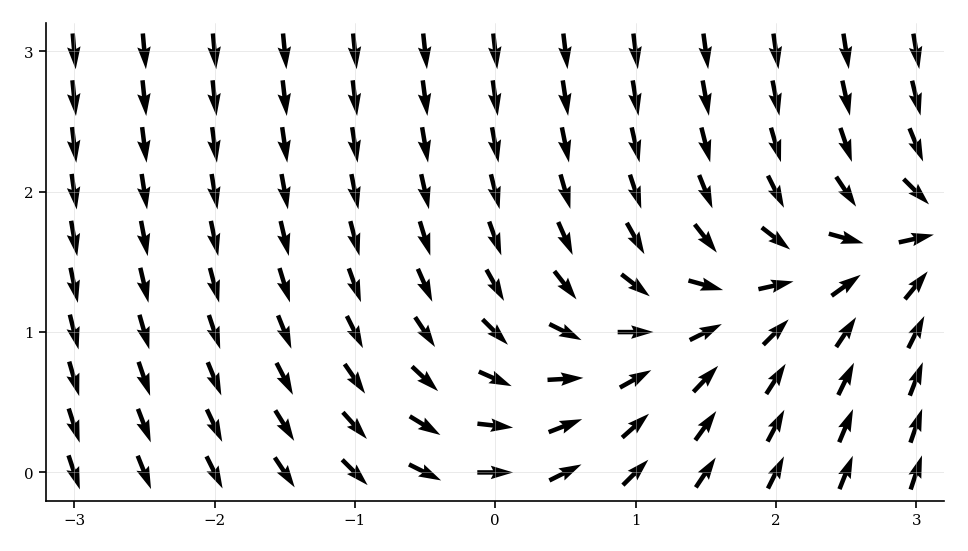
The slope field for , for , excluding , is shown below.
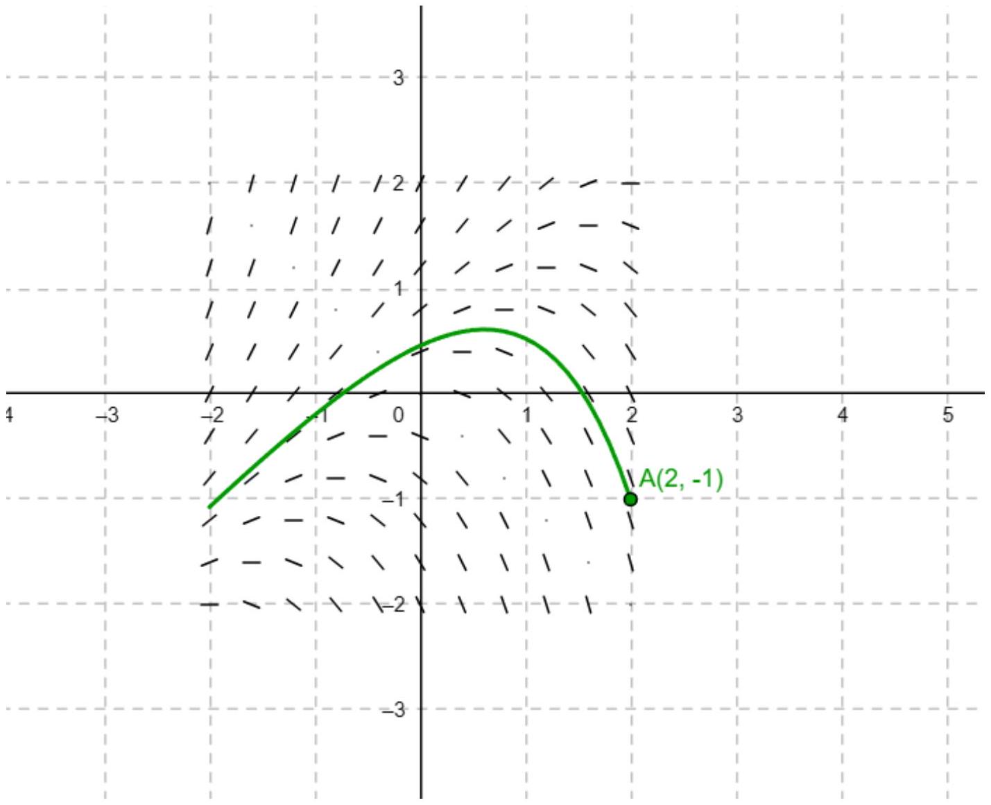
1.[2]
Find the equation of the curve where .
2.[2]
Sketch the curve from Part 1 on the slope field.
3.[2]
Sketch the solution curve through .
4.[3]
Use Euler's method with step size to approximate at .
5.[3]
Determine the coordinates of the intersection of the solution curve through with the curve from Part 1.
6.[4]
Analyze the behavior of the solution curve as .
Question 2
HLPaper 2
An object is placed into the top of a long vertical tube filled with a thick viscous fluid at time seconds.
Initially, it is thought that the resistance of the fluid would be proportional to the velocity of the object. The following model was proposed, where the object’s displacement, , from the top of the tube, measured in metres, is given by the differential equation
The maximum velocity approached by the object as it falls is known as the terminal velocity.
An experiment is performed in which the object is placed in the fluid on a number of occasions and its terminal velocity recorded. It is found that the terminal velocity was consistently smaller than that predicted by the model used. It was suggested that the resistance to motion is actually proportional to the velocity squared and so the following model was set up:
At terminal velocity, the acceleration of an object is equal to zero.
1.[7]
By substituting into the equation, find an expression for the velocity of the object at time . Give your answer in the form .
2.[2]
From your solution to part 1, or otherwise, find the terminal velocity of the object predicted by this model.
3.[2]
Write down the differential equation for the second model as a system of first-order differential equations.
4.[4]
Use Euler’s method, with a step length of , to find the displacement and velocity of the object when .
5.[1]
By repeated application of Euler’s method, find an approximation for the terminal velocity, to five significant figures.
6.[2]
Use the differential equation to find the exact terminal velocity for the object predicted by the second model.
7.[2]
Use your answers to parts 4, 5 and 6 to comment on the accuracy of the Euler approximation to this model.
Question 3
HLPaper 1
The differential equation is defined for in the region and .
1.[2]
Calculate the value of at the point .
2.[2]
Find the equation of the curve (isocline) where .
3.[3]
Determine the nature of the stationary points on the curve found in part (b) within the given region.
4.[3]
Find the equation of the tangent line to the solution curve at .
5.[4]
Determine the -coordinate where the solution curve through crosses the line , if it exists within the domain , using qualitative analysis.
Question 4
HLPaper 2
The slope field for , for , is shown below.
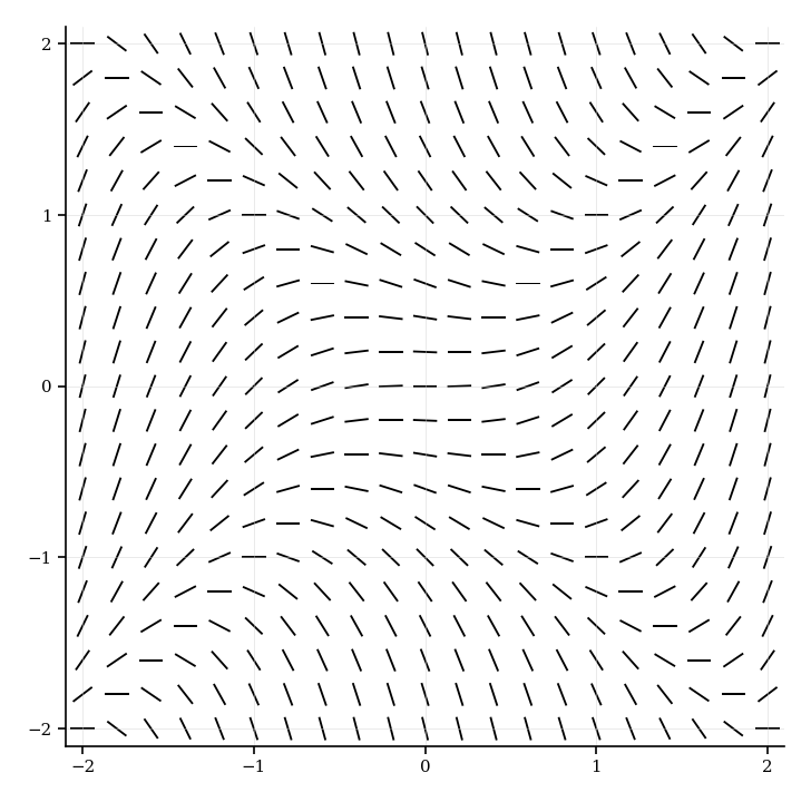
1.[2]
Find the equations of the curves where .
2.[2]
Sketch the curves from part 1 on the slope field.
3.[2]
Sketch the solution curve passing through .
4.[3]
Determine whether the solution curve from part 3 has any turning points. Justify your answer.
Question 5
HLPaper 2
The slope field for , for , is shown below.
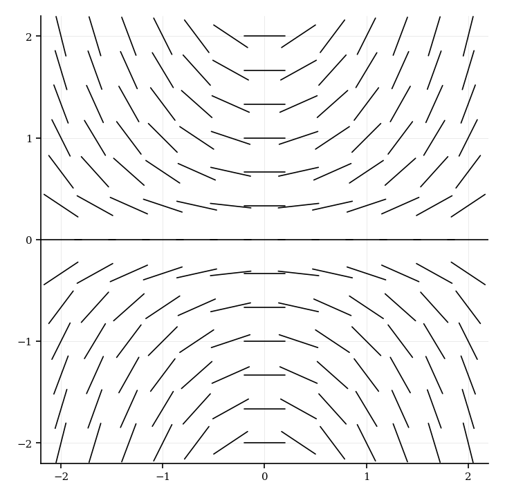
1.[2]
(a) Write down the equation of the curves where .
2.[2]
(b) Sketch the curves from part (a) on the slope field.
3.[2]
(c) Sketch the solution curve passing through .
4.[3]
(d) Determine the concavity of the solution curve from part (c) at .
Question 6
HLPaper 3
This question will investigate the solution to a coupled system of differential equations when there is only one eigenvalue.
It is desired to solve the coupled system of differential equations
The general solution to the coupled system of differential equations is hence given by
1.[7]
Show that the matrix
has only one eigenvalue. Find this eigenvalue and an associated eigenvector.
2.[5]
Hence, verify that
is a solution to the above system.
3.[5]
Verify that
is also a solution.
4.[3]
If initially at , , , find the particular solution.
5.[2]
Find the values of and when .
6.[3]
Determine the limiting value of the ratio as and hence state the equation of the line passing through the origin to which the trajectory becomes parallel.
7.[1]
State the quadrant in which the trajectory lies as and describe its motion relative to the origin.
Question 7
HLPaper 1
The diagram shows the slope field for the differential equation . The graphs of the two solutions to the differential equation that pass through points and are shown.
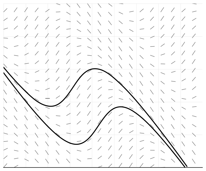
For the two solutions given, the local minimum points lie on the straight line .
1.[3]
Find the equation of , giving your answer in the form .
2.[2]
For the two solutions given, the local maximum points lie on the straight line . Find the equation of .
Question 8
HLPaper 2
The slope field for the differential equation , for , is shown below.
1.[2]
Find the equation of the curve on which the points with zero gradient lie.
2.[2]
Sketch the curve from Part 1 on the slope field above.
3.[2]
Sketch the solution curve that passes through the point .
4.[3]
Determine the coordinates of the point where the solution curve from Part 3 intersects the curve found in Part 1.
Question 9
HLPaper 3
This question will investigate the solution to a coupled system of differential equations and how to transform it to a system that can be solved by the eigenvector method. It is desired to solve the coupled system of differential equations where and represent the population of two types of symbiotic coral and is time measured in decades.
1.[2]
Find the equilibrium point for this system.
2.[3]
If initially and , use Euler's method with a time increment of 0.1 to find an approximation for the values of and when .
3.[2]
Extend this method to conjecture the limit of the ratio as .
4.[3]
Show how using the substitution transforms the system of differential equations into
5.[8]
Solve this system of equations by the eigenvalue method and hence find the general solution for of the original system.
6.[2]
Find the particular solution to the original system, given the initial conditions of part 2.
7.[2]
Hence find the exact values of and when , giving the answers to 4 significant figures.
8.[2]
Use part 6 to find limit of the ratio as .
9.[1]
With the initial conditions as given in part 2, determine if the populations converge to the equilibrium values.
10.[2]
If instead the initial conditions were given as and , find the particular solution for of the original system, in this case.
11.[2]
With the initial conditions as given in part 10, determine if the populations converge to the equilibrium values.
Question 10
HLPaper 1
Consider the differential equation for .
1.[2]
Calculate the value of at the point .
2.[2]
Find the equation of the curve where .
3.[4]
Determine the nature of the stationary points of the solution curves as they cross the curve from Part 2.
4.[2]
Find the equation of the tangent line to the solution curve passing through .
5.[4]
Analyze the behavior of the solution curve passing through as increases, identifying any asymptotic behavior.